
A model that downloads successfully can still fail when you paste a long document or open a second conversation. Its weights are only part of the memory bill. The inference engine also needs working space and a cache for the tokens being processed, while your operating system and other homelab services need room to keep running.
The useful answer to “how much memory?” starts with the exact model, its file format, your context limit and the number of requests that must run together. This guide shows how to estimate those costs, then check them on your own machine. The numbers below are calculations, not benchmarks or promises that a particular graphics card will deliver a comfortable response speed.
Featured image: original conceptual TechDecode illustration of system RAM, graphics memory and AI data.
Start with four memory budgets
Weights are the learned model parameters. They normally remain loaded across requests to the same model. The key-value, or KV, cache stores attention data for the current tokens so generation can reuse earlier work. Runtime allocations include temporary computation buffers, backend bookkeeping and, where used, compiled kernels. Host reserve covers the operating system, drivers, desktop, filesystem caching and other services.
Write a separate budget for each memory pool. With a discrete GPU, system RAM and VRAM are separate resources: spare RAM does not automatically become equally fast GPU memory. A backend may explicitly move some work or data between them. Disk space for downloads and swap is another budget; a large SSD does not make an undersized memory configuration equivalent to one that keeps its working data resident.
Also decide whether you mean one personal chat or a shared server. An idle model list is not evidence that several loaded models, a document-indexing job and multiple conversations will fit together.
Estimate weights, then read the actual file size
For an idealized model with exactly eight billion parameters, raw weight storage is parameters × bits per parameter ÷ 8. At 16 bits that is 16,000,000,000 bytes; at eight bits, 8,000,000,000; at four bits, 4,000,000,000. Decimal GB uses one billion bytes. Binary GiB uses 1,073,741,824 bytes, so those values are about 14.90, 7.45 and 3.73 GiB respectively. These are raw arithmetic examples, not complete model allocations.
Real quantization adds information needed to interpret compressed values. For example, llama.cpp’s Q4_K block stores 256 values in 144 bytes including scales and minimums: 4.5 bits per weight, despite the four-bit name. Its Q4_K_M recipe can give selected tensors higher precision. File metadata and tensors kept in other formats add further costs. Read the block definition and quantization implementation rather than treating every Q4 file as the same size.
A concrete comparison is Qwen’s Qwen3-8B Q4_K_M GGUF: the publisher metadata reports 5,027,783,488 bytes, about 5.03 GB or 4.68 GiB. That is a file size, not a VRAM measurement. Qwen describes this model as roughly 8.2 billion parameters; the “8B” name is rounded. Backend conversion or repacking can change the resident footprint.
Lower precision can change answer quality. Test your actual tasks, especially code, structured output and factual extraction. For mixture-of-experts models, use total stored parameters when estimating resident weights: Qwen3-30B-A3B has 30.5 billion total parameters and 3.3 billion activated per token. The smaller activated count does not mean its complete weights occupy a 3.3-billion-parameter footprint.
A worked KV-cache example
For a conventional dense attention cache, the raw storage estimate is 2 × layers × KV heads × head dimension × bytes per value × cached tokens × active sequences. The initial factor of two accounts for keys and values. Use KV heads, not query heads, for grouped-query attention (GQA).
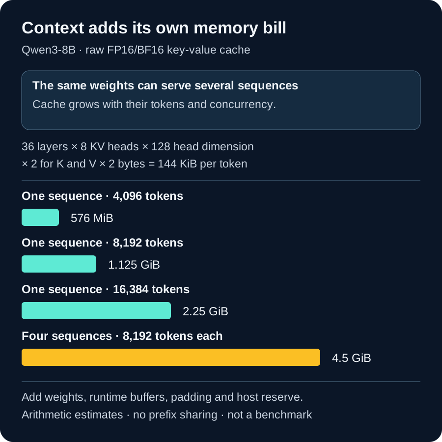
The official Qwen3-8B configuration specifies 36 layers, eight KV heads, 32 query heads and a head dimension of 128, with sliding-window attention disabled. Assuming both K and V use FP16 or BF16, each value takes two bytes. That gives 147,456 bytes, or 144 KiB, per token per sequence.
At 4,096 populated tokens, the raw cache is 576 MiB. At 8,192 it is 1.125 GiB; at 16,384, 2.25 GiB; at 32,768, 4.5 GiB. Four distinct sequences each containing 8,192 tokens also total 4.5 GiB. These estimates exclude padding, allocator overhead and working buffers, and assume no shared-prefix savings.
This small Python example reproduces the arithmetic without loading a model:
layers = 36
kv_heads = 8
head_dim = 128
bytes_per_value = 2  # FP16 or BF16 K and V
bytes_per_token = 2 * layers * kv_heads * head_dim * bytes_per_value

for tokens, sequences in [(4096, 1), (8192, 1), (16384, 1), (32768, 1), (8192, 4)]:
    cache_bytes = bytes_per_token * tokens * sequences
    print(tokens, sequences, f"{cache_bytes / (2 ** 30):.4f} GiB")
Do not reuse this formula unchanged for every architecture. Sliding-window, hybrid or compressed attention can store different data. Quantized weights also do not automatically make the KV cache four-bit; cache precision is a separate backend setting.
Context and concurrency change the answer
Count system instructions, conversation history, retrieved passages and the new prompt, then leave room for generated tokens. A 7,000-token input plus a planned 2,000-token output needs a budget beyond 8,192 tokens. Reasoning tokens can consume that budget too. Count with the model’s tokenizer or backend usage reporting; characters and words are unreliable substitutes.
A maximum context setting may allocate more than the tokens currently used. Transformers documents dynamic caches that grow, static caches that reserve a maximum, and separate quantized or CPU-offloaded cache options. These choices involve compatibility and performance tradeoffs. A smaller cache datatype is not a universal quality-neutral switch.
Several chats can usually share one loaded weight set inside one model-serving process, while retaining their own cache data. Separate worker processes or replicas may duplicate weights. Backends using paged attention can manage blocks and share eligible prefixes, but capacity planning should not assume every request has a reusable prefix.
Batch size is also not simply the number of people connected. Prompt-processing microbatches affect temporary buffers; a scheduler can batch tokens from multiple requests. Check the backend version’s meaning of context, parallel slots and batch settings. For example, the reviewed llama.cpp server documentation distinguishes logical batches, physical microbatches and parallel slots. Confirm effective per-request limits in its startup logs.
CPU, GPU offload and unified memory
A CPU backend can keep weights and cache in system RAM, provided its model format and kernels are supported. That makes existing hardware useful for evaluating a workload, but adequate capacity alone says little about response time. Processor capabilities, memory bandwidth, prompt length and backend implementation all matter.
With full GPU placement, allow VRAM for weights, cache and runtime buffers, plus the driver and other GPU users. Host RAM is still needed for the service and its loading path. Some loaders memory-map files; others allocate or convert tensors. Peak loading memory can differ from the settled allocation, so check both.
Partial GPU offload keeps some model data on the CPU and some on the GPU. llama.cpp exposes layer-placement controls, but layers are not necessarily equal in size. CPU work and transfers can limit performance. Cache placement is another decision: a GPU-loaded model can still have an explicitly offloaded cache in a backend that supports it. Inspect the placement logs rather than assuming all available memory forms one automatic pool.
On Apple silicon, compatible software such as Apple’s MLX can use shared unified memory for CPU and GPU operations. A 32 GiB unified-memory system has one physical pool; it does not provide 32 GiB of RAM plus another 32 GiB of VRAM. The OS and other applications use it too, and backend or GPU allocation limits can constrain what is usable. Other integrated GPUs also need platform-specific checks; “shared memory” does not establish identical support or speed.
For a homelab VM or container, size both the guest’s host-memory allowance and any GPU assignment. Increasing an LXC memory limit does not enlarge a discrete GPU’s VRAM. Keep the host’s other services responsive while you evaluate the inference workload.
Turn the estimate into a plan
This table combines the verified Qwen3-8B Q4_K_M file size with the raw two-byte cache estimate. It is an arithmetic starting point, not an exact sum of resident tensors or a minimum advertised GPU capacity. All rows need additional runtime and host headroom.
| Workload assumption | File + raw KV baseline | Planning implication |
|---|---|---|
| One sequence, 4,096 tokens | About 5.24 GiB | Measure loading and prompt-processing peaks before approving a small memory pool. |
| One sequence, 8,192 tokens | About 5.81 GiB | Check the configured cache allocation, output budget and desktop GPU use. |
| One sequence, 32,768 tokens | About 9.18 GiB | The raw cache is almost as large as the model file; plan for sustained usage. |
| Four sequences, 8,192 tokens each | About 9.18 GiB | Validate concurrency, scheduler buffers and whether workers duplicate weights. |
Do not add a universal “two gigabytes extra” and call the result guaranteed. Start with your measured idle usage, retain space for the largest observed runtime peak, and leave a margin for ordinary workload variation. On a shared host, include the peak needs of DNS, storage, automation and other services. Plan within the guest’s limit as well as the physical host’s capacity.
If the budget is tight, first reduce the intended context or concurrent requests. Consider a smaller model, a different quantization or supported partial offload, then reevaluate quality and responsiveness. Keeping a large model alive through heavy swapping may produce an unusable service even when it avoids an immediate error.
Measure the workload you intend to use
Record the exact model revision, quantized filename, backend build, cache dtype, context limit, GPU placement and concurrency. This makes a successful configuration repeatable and explains why two people reporting “the same 8B model” may see different memory usage.
- Establish an idle baseline. Note available host memory and GPU memory with normal services running.
- Load one model. Read logs for actual tensor placement, cache allocation and any CPU fallback. Watch the loading peak as well as settled usage.
- Exercise a representative prompt. Use non-sensitive text near your planned input length and allow the output length you need. Watch prompt processing and generation separately.
- Add intended concurrency. Evaluate the number of simultaneous requests you plan to permit, not just several open browser tabs.
- Retest after changes. A backend upgrade, new model format or larger document budget can change the result.
For a supported NVIDIA system with its driver tools installed, this read-only snapshot reports GPU memory counters:
nvidia-smi --query-gpu=memory.total,memory.used,memory.free --format=csv
NVIDIA documents these query fields. A single snapshot can miss peaks, and driver accounting has platform limitations. Compare repeated observations with backend logs and your OS monitor. On Linux, the kernel’s smaps_rollup information can help distinguish a process’s resident memory from its proportional share of shared mappings. Virtual address space alone is not the physical RAM bill.
If sharing diagnostics for help, provide settings and memory totals while redacting usernames, paths containing private details, API keys, prompts and documents. You normally do not need to upload confidential inputs to explain an out-of-memory error.
Allow for extra models and failure modes
A text-only estimate is incomplete for vision or audio. Supported multimodal setups may load an encoder or projector, process image or audio inputs in temporary buffers, and turn those inputs into model tokens. The reviewed llama.cpp multimodal documentation uses an additional projector file and controls its GPU placement. Image resolution, number of images and audio duration can therefore change the requirement. Measure a representative input rather than treating one attached photo as a fixed cost.
Document search can also add an embedding model, a reranker and a vector database. Speculative decoding can load a draft model. Decide which services must remain resident together and include their separate budgets.
When a model fails at load time, check the format, backend support and placement before assuming more memory is the only solution. Failure only on long prompts points toward cache or prompt-processing pressure; failure under concurrent requests suggests shared capacity or worker duplication. A host OOM kill and a GPU allocation error identify different pools. Reduce one setting at a time and keep the last working configuration.
Choose the smallest configuration that answers your actual questions reliably within the response time you can accept. Save the exact model identity and settings alongside your observations before buying hardware. For the service layer, the related LocalAI in Your Homelab guide covers model configuration and operation; use this memory budget to decide what that service can reasonably host.